
Chapter 20 Masking HR data
In the toolbox of every HR Analytics expert, the ability to quickly anonymize data for test and development environments finds an important place. Surely you want to be able to protect confidential data from inappropriate views.
Ensure all needed libraries are installed
library(tidyverse)
library(randNames)
library(smoothmest)
20.0.1 Whitehouse dataset
Load a data set with first and last names and let us preview the dataset
whitehouse <- read_csv("https://hranalytics.netlify.com/data/2016-Report-White-House-Staff.csv")Let us replace original names with fake names
#Create a set of new names of equal length as the original dataset

fake <- nrow(whitehouse) %>%
  rand_names (nat="US")

#Function to capitalise the first letter
firstup <- function(x) {
  substr(x, 1, 1) <- toupper(substr(x, 1, 1))
  x
}

#Create a dataframe without the original names columns
whitehouse_with_no_names <- dplyr::select(whitehouse, -Name)

#Create a column of fake last and first names
fake$newnames <- paste0(firstup(fake$name.last), ", ", firstup(fake$name.first))

#Create a column of fake last and first names of exactly the length of the data frame without the original names
result <- fake[1:nrow(whitehouse_with_no_names),]

#Bind the dataset without names with the new dataset containing fake names
whitehouse_masked <- cbind(result$newnames, whitehouse_with_no_names)

#Rename the column title to "Name"
colnames(whitehouse_masked)[1] <- "Name"
Let us replace original names with random numbers
# Set seed for reproducibility of the random numbers
set.seed(42)

# Replace names with random numbers from 1 to 1000
whitehouse_no_names <- whitehouse_masked %>%
  mutate(Name = sample(1:1000, nrow(whitehouse_masked)))
Let us anonymise the salary data
We can use four different methods to anonymise data: * Rounding Salary to the nearest ten thousand * Top coding consists of bringing data to an upper limit. * Bottom coding consists of bringing data to a lower limit.
In data analysis exists various types of transformations, reciprocal, logarithm, cube root, square root and square, however in the following we will demonstrate only the square root transformation.
# Rounding Salary to the nearest ten thousand
whitehouse_no_identifiers <- whitehouse_no_names %>%
  mutate(Salary = round(Salary, digits = -4))

# Top coding convert the salaries into three categories
whitehouse.gen <- whitehouse_masked %>%
  mutate(Salary = ifelse(Salary < 50000, 0,
                         ifelse(Salary >= 50000 & Salary < 100000, 1, 2)))

# Bottom Coding
whitehouse.bottom <- whitehouse_masked %>%
  mutate(Salary = ifelse(Salary<=45000, 45000, Salary))
20.0.2 Fertility dataset
Let us explore deeper anonymisation option of generating synthetic data. We will do on the basis of the fertility dataset available from UCI website: https://archive.ics.uci.edu/ml/datasets/Fertility
UCI logo
It needs to be loaded first and let us preview it.
fertility <- read_csv("https://https://hranalytics.netlify.com/data/fertility_Diagnosis.txt", col_names = FALSE)# Let us assign significant column titles
colnames(fertility) <- c("Season", "Age", "Child_Disease", "Accident_Trauma", "Surgical_Intervention","High_Fevers", "Alcohol_Consumption","Smoking_Habit","Hours_Sitting","Diagnosis")
# View fertility data
fertility# A tibble: 100 x 10
Season Age Child_Disease Accident_Trauma Surgical_Interv~ High_Fevers
<dbl> <dbl> <dbl> <dbl> <dbl> <dbl>
1 -0.33 0.69000 0 1 1 0
2 -0.33 0.94 1 0 1 0
3 -0.33 0.5 1 0 0 0
4 -0.33 0.75 0 1 1 0
5 -0.33 0.67 1 1 0 0
6 -0.33 0.67 1 0 1 0
7 -0.33 0.67 0 0 0 -1
8 -0.33 1 1 1 1 0
9 1 0.64 0 0 1 0
10 1 0.61 1 0 0 0
# ... with 90 more rows, and 4 more variables: Alcohol_Consumption <dbl>,
# Smoking_Habit <dbl>, Hours_Sitting <dbl>, Diagnosis <chr>Let us examine the dataset.
More on the data attributes is availalble here: https://archive.ics.uci.edu/ml/datasets/Fertility
# Number of participants with Surgical_Intervention and Diagnosis
fertility %>%
  group_by(Diagnosis) %>%
  summarise_at(vars(Surgical_Intervention), sum)
# A tibble: 2 x 2
Diagnosis Surgical_Intervention
<chr> <dbl>
1 N 44
2 O 7# Number of participants with Surgical_Intervention and Diagnosis
fertility %>%
summarise_at(vars(Age), funs(mean, sd))# A tibble: 1 x 2
mean sd
<dbl> <dbl>
1 0.669 0.121319# Counts of the Groups in High_Fevers
fertility %>%
count(High_Fevers)# A tibble: 3 x 2
High_Fevers n
<dbl> <int>
1 -1 9
2 0 63
3 1 28# Counts of the Groups in Child_Disease and Accident_Trauma
fertility %>%
count(Child_Disease,Accident_Trauma)# A tibble: 4 x 3
Child_Disease Accident_Trauma n
<dbl> <dbl> <int>
1 0 0 10
2 0 1 3
3 1 0 46
4 1 1 41# Calculate the average of Child_Disease
fertility %>%
summarise_at(vars(Child_Disease), mean)# A tibble: 1 x 1
Child_Disease
<dbl>
1 0.87In the following we will generate synthetic data sampling from a normal distribution through the subsequent steps: 1. First create a new dataset called “fert,” after applying a log transformation on the hours sitting variable. 2. Calculate the average and the standard deviation 3. Set a seed for reproducibility 4. Generate new data normally distributed for the hours sitting variable 5. Retransform back the log variable using exponential. 6. Hard bound data not falling in the right range 7. Recheck the range. 8. Substitute the synthtic data back into the initial fert dataset.
fert <- fertility %>%
    mutate(Hours_Sitting = log(Hours_Sitting))

fert %>%
    summarise_at(vars(Hours_Sitting), funs(mean, sd))
# A tibble: 1 x 2
mean sd
<dbl> <dbl>
1 -1.01224 0.504779set.seed(42)
hours.sit <- rnorm(100, -1.01, 0.50)
hours.sit <- exp(hours.sit)
hours.sit[hours.sit < 0] <- 0
hours.sit[hours.sit > 1] <- 1
range(hours.sit)[1] 0.0815 1.0000fert$Hours_Sitting <- hours.sitIn data analysis exists various types of transformations, reciprocal, logarithm, cube root, square root and square, however in the following we will demonstrate only the square root transformation.
# Square root Transformation of Salary
whitehouse.salary <- whitehouse_masked %>%
  mutate(Salary = sqrt(Salary))

# Calculate the mean and standard deviation
stats <- whitehouse.salary %>%
  summarise_at(vars(Salary), funs(mean, sd))

# Generate Synthetic data with the same mean and standard deviation
salary_transformed <- rnorm(nrow(whitehouse_masked), mean(whitehouse.salary$Salary), sd(whitehouse.salary$Salary))

# Power transformation
salary_original <- salary_transformed^2

# Hard bound
salary <- ifelse(salary_original < 0, 0, salary_original)
Let us introduce now the concept of differential privacy, a mathematical concept used by big names like Google, Census Bureau and Apple. Why Differential Privacy? It quantifies the privacy loss via a privacy budget, called epsilon. It assumes the worst-case scenario about the data intruder. Smaller privacy budget means less information or a noiser answer, however epsilon cannot be zero or lower.
Global Sensitivity of Other Queries n is total number of observations a is the lower bound of the data b is the upper bound of the data Counting: 1 Proportion: 1 / n Mean: (b - a) / n
small global sensitivity results in less noise large global sensitivity results in more noise
Number of observations n <- nrow(fertility)
Global sensitivity of counts gs.count <- 1
Global sensitivity of proportions gs.prop <- 1/n
Lower bound a <- 0
Upper bound b <- 1
Global sensitivity of mean gs.mean <- (b - a) / n
Global sensitivity of proportions gs.var <- (b - a)^2 / n
fertility %>%
    summarise_at(vars(Child_Disease), sum)
# A tibble: 1 x 1
Child_Disease
<dbl>
1 87library(smoothmest)
#rdoublex(draws, mean, shaping)
#rdoublex is a random number generator. It creates a vector of random numbers generated by the double exponential distribution.The double exponential distribution is also commonly referred to as the Laplace distribution. The following is the plot of the double exponential probability density function.
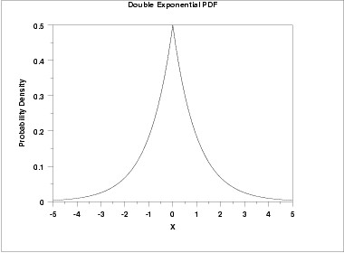
plot of double exponential probability density function
set.seed(42)

rdoublex(1, 87, 1 / 10)
[1] 87#[1] 87.01983
set.seed(42)
rdoublex(1, 87, 1 / 0.1)[1] 85#[1] 88.98337Sequential Composition
Suppose a set of privacy mechanisms M are sequentially performed on a dataset, and each M provides the max epsilon privacy guarantee.
The sequential composition undertakes the privacy guarantee for a sequence of differentially private computations. When a set of randomized mechanisms has been performed sequentially on a dataset, the final privacy guarantee is determined by the summation of total privacy budgets.
The privacy budget must be divided by two.
#Set Value of Epsilon
eps <- 0.1 / 2

# GS of Mean and Variance
gs.mean <- 0.01
gs.var <- 0.01

# Apply the Laplace mechanism
set.seed(42)
rdoublex(1, 0.41, gs.mean / eps)
[1] 0.37#[1] 0.4496674
rdoublex(1, 0.19, gs.var / eps)[1] 0.247#[1] 0.2466982Parallel Composition
Suppose a set of privacy mechanisms M are sequentially performed on a dataset, and each M provides the sum epsilon privacy guarantee.
The sequential composition undertakes the privacy guarantee for a sequence of differentially private computations. When a set of randomized mechanisms has been performed sequentially on a dataset, the final privacy guarantee is determined by the summation of total privacy budgets.
The privacy budget does not need to be divided. The query with the most epsilon is the budget for the data.
#High_Fevers and Mean of Hours_Sitting

fertility %>%
  filter(High_Fevers >= 0) %>%
  summarise_at(vars(Hours_Sitting), mean)
# A tibble: 1 x 1
Hours_Sitting
<dbl>
1 0.393297#Hours_Sitting 0.3932967
# No High_Fevers and Mean of Hours_Sitting
fertility %>%
filter(High_Fevers == -1) %>%
summarise_at(vars(Hours_Sitting), mean)# A tibble: 1 x 1
Hours_Sitting
<dbl>
1 0.543333#Hours_Sitting 0.5433333
#Set Value of Epsilon
eps <- 0.1
# GS of mean for Hours_Sitting
gs.mean <- 1 / 100
# Apply the Laplace mechanism
set.seed(42)
rdoublex(1, 0.39, gs.mean / eps)[1] 0.37#[1] 0.4098337
rdoublex(1, 0.54, gs.mean / eps)[1] 0.568#[1] 0.5683491Prepping up data
# Set Value of Epsilon
eps <- 0.01
# GS of counts
gs.count <- 1

fertility %>%
  count(Smoking_Habit)
# A tibble: 3 x 2
Smoking_Habit n
<dbl> <int>
1 -1 56
2 0 23
3 1 21#Smoking Count
#-1 56
# 0 23
# 1 21
#Apply the Laplace mechanism
set.seed(42)
smoking1 <- rdoublex(1, 56, gs.count / eps / 2) %>%
round()
smoking2 <- rdoublex(1, 23, gs.count / eps / 2) %>%
round()
# Post-process based on previous queries
smoking3 <- nrow(fertility) - smoking1 - smoking2
# Checking the noisy answers
smoking1[1] 46#[1] 60
smoking2[1] 37#[1] 29
smoking3[1] 17#[1] 11Impossible and Inconsistent Answers
# Set Value of Epsilon
eps <- 0.01
# GS of counts
gs.count <- 1

# Display Participants with Abnormal Diagnosis
Number_abnormal <- fertility %>% filter(Diagnosis=="O") %>% summarise(sum_x1 = sum(Diagnosis=="O"))

#Negative Counts: Applying the Laplace mechanism
# Apply the Laplace mechanism and set.seed(22)
set.seed(22)
rdoublex(1, 12, gs.count / eps) %>%
  round()
[1] -79#[1] -79
# Apply the Laplace mechanism and set.seed(22)
set.seed(22)
rdoublex(1, 12, gs.count / eps) %>%
round() %>%
max(0)[1] 0#[1] 0
# Suppose we set a different seed
set.seed(12)
noisy_answer <- rdoublex(1, 12, gs.count / eps) %>%
round() %>%
max(0)
n <- nrow(fertility)
# ifelse example
ifelse(noisy_answer > n, n, noisy_answer)[1] 100#[1] 100
#Normalising
# Set Value of Epsilon
eps <- 0.01
# GS of Counts
gs.count <- 1
fertility %>%
count(Smoking_Habit)# A tibble: 3 x 2
Smoking_Habit n
<dbl> <int>
1 -1 56
2 0 23
3 1 21#Smoking Count
# -1 56
# 0 23
# 1 21
# Apply the Laplace mechanism and set.seed(42)
set.seed(42)
smoking1 <- rdoublex(1, 56, gs.count / eps / 2) %>%
max(0)
smoking2 <- rdoublex(1, 23, gs.count / eps / 2) %>%
max(0)
smoking3 <- rdoublex(1, 21, gs.count / eps / 2) %>%
max(0)
# Checking the noisy answers
smoking <- c(smoking1, smoking2, smoking3)
smoking[1] 46.1 37.2 44.7#[1] 65.91684 37.17455 0.00000
# Normalize smoking
normalized <- (smoking/sum(smoking)) * (nrow(fertility))
# Round the values
round(normalized)[1] 36 29 35#[1] 64 36 0